I'm currently trying to use the VLOOKUP function across multiple sheets, which isn't an issue. The problem i'm facing, is that i need to sum the cells across the sheets.
I cant find a way to SUM the cells without having multiple errors. The REAL problem is, i'm a complete novice. I am highly likely using the complete wrong formulas!
=SUMPRODUCT(VLOOKUP(B2,December!A2:B88,{1,2},FALSE))*SUMPRODUCT(VLOOKUP(B2,November!A2:B90,{1,2},FALSE))
^This is the current formula im working on, and ive made an example workbook for the purpose of discretion.
Client1 $130 Client2 $520 Client3 $100 Client4 $240 Client5 $880
^December
Client1 $130 Client2 $520 Client3 $100 Client4 $240 Client5 $880
^November
What i would like to do, is be able to write in the clients name, and a YTD pop up with the sum of all their fees.
Thank you greatly in advance, for i am truly lost!
UPDATE!
I worked out that i had used an asterisk instead of a +(silly me) and was able to get the total for a few months, however i'm trying to get 6 months of data together and now its just coming up with #N/A
=SUMPRODUCT(VLOOKUP(B2,December!A2:B88,{1,2},FALSE))+SUMPRODUCT(VLOOKUP(B2,November!A2:B92,{1,2},FALSE))+SUMPRODUCT(VLOOKUP(B2,October!A2:B86,{1,2},FALSE))+SUMPRODUCT(VLOOKUP(B2,September!A2:B78,{1,2},FALSE))+SUMPRODUCT(VLOOKUP(B2,August!A2:B82,{1,2},FALSE))+SUMPRODUCT(VLOOKUP(B2,July!A2:B85,{1,2},FALSE))
^current formula
This thread is locked. You can follow the question or vote as helpful, but you cannot reply to this thread. |
I cant find a way to SUM the cells without having multiple errors. The REAL problem is, i'm a complete novice. I am highly likely using the complete wrong formulas!
=SUMPRODUCT(VLOOKUP(B2,December!A2:B88,{1,2},FALSE))*SUMPRODUCT(VLOOKUP(B2,November!A2:B90,{1,2},FALSE))
^This is the current formula im working on, and ive made an example workbook for the purpose of discretion.
| Client1 | $130 |
| Client2 | $520 |
| Client3 | $100 |
| Client4 | $240 |
| Client5 | $880 |
^December
| Client1 | $130 |
| Client2 | $520 |
| Client3 | $100 |
| Client4 | $240 |
| Client5 | $880 |
^November
What i would like to do, is be able to write in the clients name, and a YTD pop up with the sum of all their fees.
Thank you greatly in advance, for i am truly lost!
UPDATE!
I worked out that i had used an asterisk instead of a +(silly me) and was able to get the total for a few months, however i'm trying to get 6 months of data together and now its just coming up with #N/A
=SUMPRODUCT(VLOOKUP(B2,December!A2:B88,{1,2},FALSE))+SUMPRODUCT(VLOOKUP(B2,November!A2:B92,{1,2},FALSE))+SUMPRODUCT(VLOOKUP(B2,October!A2:B86,{1,2},FALSE))+SUMPRODUCT(VLOOKUP(B2,September!A2:B78,{1,2},FALSE))+SUMPRODUCT(VLOOKUP(B2,August!A2:B82,{1,2},FALSE))+SUMPRODUCT(VLOOKUP(B2,July!A2:B85,{1,2},FALSE))
^current formula
Replies (8)
Although what you are looking for is feasible, it involves quite complicating array formulation and not easy for most user to maintain or for the file to pass to other people...
To simplify your problem, I would highly recommend you change how you store your data on your workbook.
Instead of having data of individual months on individual sheets, put them all in a tabular format on a worksheet, e.g. Year, Month, Client, Value... to be on Column A:D respectively.
In this way, you may get your answer very quickly with either SUMIF, or even better a Pivot Table.
Was this reply helpful?
Have you checked the following:
1. Check if all the worksheets which you are using in your formula exists in your workbook
2. Check if there is any spelling difference in the names of your worksheets
Excel is Awesome!! One problem always has multiple solutions.
If my answer solves your problem, please tick mark it as Answered.
Cheers RajeshC 2 people found this reply helpful
· Was this reply helpful?
Yes! the names were different!!!!
However, ive encountered a second issue when i went on to the second column..... Is it possible to use a cell 'G2', when in the cell, there is already a formula present? '=SUM(D2+E2+F2)'
Was this reply helpful?
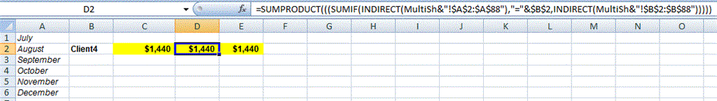
Given below are 2 options:
Option 1: Create a named range MultiSh: in the Name Manager click New & name it MultiSh > in the Refers To box enter ={"July","August","September","October","November","December"}
Enter below formula:
=SUMPRODUCT(((SUMIF(INDIRECT(MultiSh&"!$A$2:$A$88"),"="&$B$2,INDIRECT(MultiSh&"!$B$2:$B$88")))))
Refer below image:
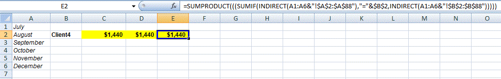
Option 2: Enter the months in range A1:A6 - July, August, September, October, November, December
Use this formula:
=SUMPRODUCT(((SUMIF(INDIRECT(A1:A6&"!$A$2:$A$88"),"="&$B$2,INDIRECT(A1:A6&"!$B$2:$B$88")))))
Refer below image:
Regards,
Amit Tandon
If this response answers your question then please mark as Answer.
1 person found this reply helpful
· Was this reply helpful?
Can someone tell me an easier way to write this.
=IFERROR(SUMPRODUCT(VLOOKUP(B7,December!A1:G93,{1,7},FALSE))+SUMPRODUCT(VLOOKUP(B7,November!A1:G97,{1,7},FALSE))+SUMPRODUCT(VLOOKUP(B7,October!A1:G91,{1,7},FALSE))+SUMPRODUCT(VLOOKUP(B7,September!A1:G83,{1,7},FALSE))+SUMPRODUCT(VLOOKUP(B7,August!A1:G87,{1,7},FALSE))+SUMPRODUCT(VLOOKUP(B7,July!A1:G90,{1,7},FALSE))),(SUMPRODUCT(VLOOKUP(B7,December!A1:G93,{1,7},FALSE))+SUMPRODUCT(VLOOKUP(B7,November!A1:G97,{1,7},FALSE))+SUMPRODUCT(VLOOKUP(B7,October!A1:G91,{1,7},FALSE))+SUMPRODUCT(VLOOKUP(B7,September!A1:G83,{1,7},FALSE))+SUMPRODUCT(VLOOKUP(B7,August!A1:G87,{1,7},FALSE))),IFERROR(SUMPRODUCT(VLOOKUP(B7,December!A1:G93,{1,7},FALSE))+SUMPRODUCT(VLOOKUP(B7,November!A1:G97,{1,7},FALSE))+SUMPRODUCT(VLOOKUP(B7,October!A1:G91,{1,7},FALSE))+SUMPRODUCT(VLOOKUP(B7,September!A1:G83,{1,7},FALSE))+SUMPRODUCT(VLOOKUP(B7,August!A1:G87,{1,7},FALSE))),(SUMPRODUCT(VLOOKUP(B7,December!A1:G93,{1,7},FALSE))+SUMPRODUCT(VLOOKUP(B7,November!A1:G97,{1,7},FALSE))+SUMPRODUCT(VLOOKUP(B7,October!A1:G91,{1,7},FALSE))+SUMPRODUCT(VLOOKUP(B7,September!A1:G83,{1,7},FALSE))),IFERROR(SUMPRODUCT(VLOOKUP(B7,December!A1:G93,{1,7},FALSE))+SUMPRODUCT(VLOOKUP(B7,November!A1:G97,{1,7},FALSE))+SUMPRODUCT(VLOOKUP(B7,October!A1:G91,{1,7},FALSE))+SUMPRODUCT(VLOOKUP(B7,September!A1:G83,{1,7},FALSE))),(SUMPRODUCT(VLOOKUP(B7,December!A1:G93,{1,7},FALSE))+SUMPRODUCT(VLOOKUP(B7,November!A1:G97,{1,7},FALSE))+SUMPRODUCT(VLOOKUP(B7,October!A1:G91,{1,7},FALSE))),IFERROR(SUMPRODUCT(VLOOKUP(B7,December!A1:G93,{1,7},FALSE))+SUMPRODUCT(VLOOKUP(B7,November!A1:G97,{1,7},FALSE))+SUMPRODUCT(VLOOKUP(B7,October!A1:G91,{1,7},FALSE))),(SUMPRODUCT(VLOOKUP(B7,December!A1:G93,{1,7},FALSE))+SUMPRODUCT(VLOOKUP(B7,November!A1:G97,{1,7},FALSE))),IFERROR(SUMPRODUCT(VLOOKUP(B7,December!A1:G93,{1,7},FALSE))+SUMPRODUCT(VLOOKUP(B7,November!A1:G97,{1,7},FALSE))),(SUMPRODUCT(VLOOKUP(B7,December!A1:G93,{1,7},FALSE)))
If its not obvious what im trying to do..... i want the formula to eliminate a month if the client is not applicable for that month.
for example, if Client1 wasnt a client in November, i want the formula to recognize this and just look in the months Client1 is in.
Please don't yell at me for my bad formula creation, i have only JUST started using formula's for the business XD
It worked until september, then it just said too many arguments.
Someone has already suggested a different layout for my graph, and that is simply not possible.
PLEASE HELP!
Was this reply helpful?
Can someone tell me an easier way to write this.
=IFERROR(SUMPRODUCT(VLOOKUP(B7,December!A1:G93,{1,7},FALSE))+SUMPRODUCT(VLOOKUP(B7,November!A1:G97,{1,7},FALSE))+SUMPRODUCT(VLOOKUP(B7,October!A1:G91,{1,7},FALSE))+SUMPRODUCT(VLOOKUP(B7,September!A1:G83,{1,7},FALSE))+SUMPRODUCT(VLOOKUP(B7,August!A1:G87,{1,7},FALSE))+SUMPRODUCT(VLOOKUP(B7,July!A1:G90,{1,7},FALSE))),(SUMPRODUCT(VLOOKUP(B7,December!A1:G93,{1,7},FALSE))+SUMPRODUCT(VLOOKUP(B7,November!A1:G97,{1,7},FALSE))+SUMPRODUCT(VLOOKUP(B7,October!A1:G91,{1,7},FALSE))+SUMPRODUCT(VLOOKUP(B7,September!A1:G83,{1,7},FALSE))+SUMPRODUCT(VLOOKUP(B7,August!A1:G87,{1,7},FALSE))),IFERROR(SUMPRODUCT(VLOOKUP(B7,December!A1:G93,{1,7},FALSE))+SUMPRODUCT(VLOOKUP(B7,November!A1:G97,{1,7},FALSE))+SUMPRODUCT(VLOOKUP(B7,October!A1:G91,{1,7},FALSE))+SUMPRODUCT(VLOOKUP(B7,September!A1:G83,{1,7},FALSE))+SUMPRODUCT(VLOOKUP(B7,August!A1:G87,{1,7},FALSE))),(SUMPRODUCT(VLOOKUP(B7,December!A1:G93,{1,7},FALSE))+SUMPRODUCT(VLOOKUP(B7,November!A1:G97,{1,7},FALSE))+SUMPRODUCT(VLOOKUP(B7,October!A1:G91,{1,7},FALSE))+SUMPRODUCT(VLOOKUP(B7,September!A1:G83,{1,7},FALSE))),IFERROR(SUMPRODUCT(VLOOKUP(B7,December!A1:G93,{1,7},FALSE))+SUMPRODUCT(VLOOKUP(B7,November!A1:G97,{1,7},FALSE))+SUMPRODUCT(VLOOKUP(B7,October!A1:G91,{1,7},FALSE))+SUMPRODUCT(VLOOKUP(B7,September!A1:G83,{1,7},FALSE))),(SUMPRODUCT(VLOOKUP(B7,December!A1:G93,{1,7},FALSE))+SUMPRODUCT(VLOOKUP(B7,November!A1:G97,{1,7},FALSE))+SUMPRODUCT(VLOOKUP(B7,October!A1:G91,{1,7},FALSE))),IFERROR(SUMPRODUCT(VLOOKUP(B7,December!A1:G93,{1,7},FALSE))+SUMPRODUCT(VLOOKUP(B7,November!A1:G97,{1,7},FALSE))+SUMPRODUCT(VLOOKUP(B7,October!A1:G91,{1,7},FALSE))),(SUMPRODUCT(VLOOKUP(B7,December!A1:G93,{1,7},FALSE))+SUMPRODUCT(VLOOKUP(B7,November!A1:G97,{1,7},FALSE))),IFERROR(SUMPRODUCT(VLOOKUP(B7,December!A1:G93,{1,7},FALSE))+SUMPRODUCT(VLOOKUP(B7,November!A1:G97,{1,7},FALSE))),(SUMPRODUCT(VLOOKUP(B7,December!A1:G93,{1,7},FALSE)))
If its not obvious what im trying to do..... i want the formula to eliminate a month if the client is not applicable for that month.
for example, if Client1 wasnt a client in November, i want the formula to recognize this and just look in the months Client1 is in.
Please don't yell at me for my bad formula creation, i have only JUST started using formula's for the business XD
It worked until september, then it just said too many arguments.
Someone has already suggested a different layout for my graph, and that is simply not possible.
PLEASE HELP!
In my earlier reply, I had mentioned an Option 2 wherein your enter relevant months in cells A1:A6. You may adjust this range in the formula, say if you enter A1:A5, then December will not be included & you will have to change the range from A1:A6 to A1:A5 which appears twice (marked in bold) in the formula. You may enter relevant months in a range (say A1:A3 or whatever) & change the reference within the formula. In case you want, I can upload a file which you may download to check how it works.
Option 2: Enter the months in range A1:A6 - July, August, September, October, November, December
Use this formula:
=SUMPRODUCT(((SUMIF(INDIRECT(A1:A6&"!$A$2:$A$88"),"="&$B$2,INDIRECT(A1:A6&"!$B$2:$B$88")))))
Regards,
Amit Tandon
Was this reply helpful?
If you could upload a file, that would be fantastic, as i'm not really certain what your saying...
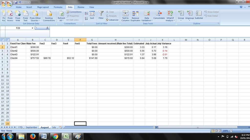
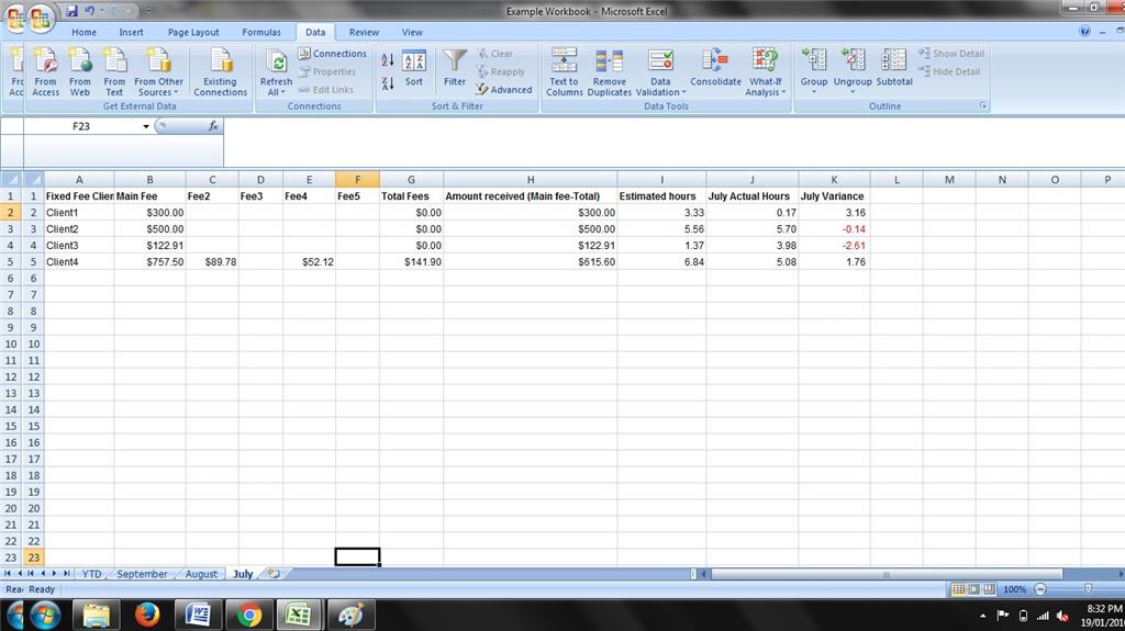
I made a sample excel that copies exactly whats in my spreadsheet without all the sensitive information, so you have a better idea of what im trying to do. Don't know how to upload, so ive attached photos :)
The formula in the first photo is the one i need to be adjusted, as it doesn't work for Client5 who only appears in September.
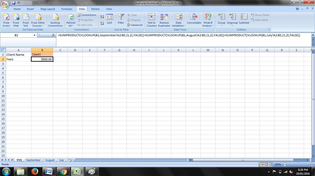
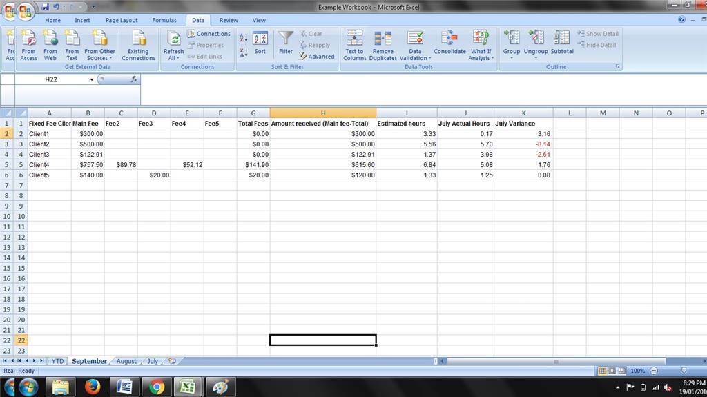
1 person found this reply helpful
· Was this reply helpful?
This is somewhat different from earlier. Have modified the formula ... please download file from below link. Have given 2 options in the tabs - YTD & YTD_1.
http://globaliconnect.com/excel/Microsoft/DownloadFiles/Vlookup_SumProduct_MultiSheets.xlsx
Was this reply helpful?
Although what you are looking for is feasible, it involves quite complicating array formulation and not easy for most user to maintain or for the file to pass to other people...
To simplify your problem, I would highly recommend you change how you store your data on your workbook.
Instead of having data of individual months on individual sheets, put them all in a tabular format on a worksheet, e.g. Year, Month, Client, Value... to be on Column A:D respectively.
In this way, you may get your answer very quickly with either SUMIF, or even better a Pivot Table.
Was this reply helpful?
Have you checked the following:
1. Check if all the worksheets which you are using in your formula exists in your workbook
2. Check if there is any spelling difference in the names of your worksheets
If my answer solves your problem, please tick mark it as Answered.
Cheers RajeshC
2 people found this reply helpful
·Was this reply helpful?
Yes! the names were different!!!!
However, ive encountered a second issue when i went on to the second column..... Is it possible to use a cell 'G2', when in the cell, there is already a formula present? '=SUM(D2+E2+F2)'
Was this reply helpful?
Given below are 2 options:
Option 1: Create a named range MultiSh: in the Name Manager click New & name it MultiSh > in the Refers To box enter ={"July","August","September","October","November","December"}
Enter below formula:
=SUMPRODUCT(((SUMIF(INDIRECT(MultiSh&"!$A$2:$A$88"),"="&$B$2,INDIRECT(MultiSh&"!$B$2:$B$88")))))
Refer below image:
Option 2: Enter the months in range A1:A6 - July, August, September, October, November, December
Use this formula:
=SUMPRODUCT(((SUMIF(INDIRECT(A1:A6&"!$A$2:$A$88"),"="&$B$2,INDIRECT(A1:A6&"!$B$2:$B$88")))))
Refer below image:
Regards,
Amit Tandon
If this response answers your question then please mark as Answer.
1 person found this reply helpful
·Was this reply helpful?
Can someone tell me an easier way to write this.
=IFERROR(SUMPRODUCT(VLOOKUP(B7,December!A1:G93,{1,7},FALSE))+SUMPRODUCT(VLOOKUP(B7,November!A1:G97,{1,7},FALSE))+SUMPRODUCT(VLOOKUP(B7,October!A1:G91,{1,7},FALSE))+SUMPRODUCT(VLOOKUP(B7,September!A1:G83,{1,7},FALSE))+SUMPRODUCT(VLOOKUP(B7,August!A1:G87,{1,7},FALSE))+SUMPRODUCT(VLOOKUP(B7,July!A1:G90,{1,7},FALSE))),(SUMPRODUCT(VLOOKUP(B7,December!A1:G93,{1,7},FALSE))+SUMPRODUCT(VLOOKUP(B7,November!A1:G97,{1,7},FALSE))+SUMPRODUCT(VLOOKUP(B7,October!A1:G91,{1,7},FALSE))+SUMPRODUCT(VLOOKUP(B7,September!A1:G83,{1,7},FALSE))+SUMPRODUCT(VLOOKUP(B7,August!A1:G87,{1,7},FALSE))),IFERROR(SUMPRODUCT(VLOOKUP(B7,December!A1:G93,{1,7},FALSE))+SUMPRODUCT(VLOOKUP(B7,November!A1:G97,{1,7},FALSE))+SUMPRODUCT(VLOOKUP(B7,October!A1:G91,{1,7},FALSE))+SUMPRODUCT(VLOOKUP(B7,September!A1:G83,{1,7},FALSE))+SUMPRODUCT(VLOOKUP(B7,August!A1:G87,{1,7},FALSE))),(SUMPRODUCT(VLOOKUP(B7,December!A1:G93,{1,7},FALSE))+SUMPRODUCT(VLOOKUP(B7,November!A1:G97,{1,7},FALSE))+SUMPRODUCT(VLOOKUP(B7,October!A1:G91,{1,7},FALSE))+SUMPRODUCT(VLOOKUP(B7,September!A1:G83,{1,7},FALSE))),IFERROR(SUMPRODUCT(VLOOKUP(B7,December!A1:G93,{1,7},FALSE))+SUMPRODUCT(VLOOKUP(B7,November!A1:G97,{1,7},FALSE))+SUMPRODUCT(VLOOKUP(B7,October!A1:G91,{1,7},FALSE))+SUMPRODUCT(VLOOKUP(B7,September!A1:G83,{1,7},FALSE))),(SUMPRODUCT(VLOOKUP(B7,December!A1:G93,{1,7},FALSE))+SUMPRODUCT(VLOOKUP(B7,November!A1:G97,{1,7},FALSE))+SUMPRODUCT(VLOOKUP(B7,October!A1:G91,{1,7},FALSE))),IFERROR(SUMPRODUCT(VLOOKUP(B7,December!A1:G93,{1,7},FALSE))+SUMPRODUCT(VLOOKUP(B7,November!A1:G97,{1,7},FALSE))+SUMPRODUCT(VLOOKUP(B7,October!A1:G91,{1,7},FALSE))),(SUMPRODUCT(VLOOKUP(B7,December!A1:G93,{1,7},FALSE))+SUMPRODUCT(VLOOKUP(B7,November!A1:G97,{1,7},FALSE))),IFERROR(SUMPRODUCT(VLOOKUP(B7,December!A1:G93,{1,7},FALSE))+SUMPRODUCT(VLOOKUP(B7,November!A1:G97,{1,7},FALSE))),(SUMPRODUCT(VLOOKUP(B7,December!A1:G93,{1,7},FALSE)))
If its not obvious what im trying to do..... i want the formula to eliminate a month if the client is not applicable for that month.
for example, if Client1 wasnt a client in November, i want the formula to recognize this and just look in the months Client1 is in.
Please don't yell at me for my bad formula creation, i have only JUST started using formula's for the business XD
It worked until september, then it just said too many arguments.
Someone has already suggested a different layout for my graph, and that is simply not possible.
PLEASE HELP!
Was this reply helpful?
Can someone tell me an easier way to write this.
=IFERROR(SUMPRODUCT(VLOOKUP(B7,December!A1:G93,{1,7},FALSE))+SUMPRODUCT(VLOOKUP(B7,November!A1:G97,{1,7},FALSE))+SUMPRODUCT(VLOOKUP(B7,October!A1:G91,{1,7},FALSE))+SUMPRODUCT(VLOOKUP(B7,September!A1:G83,{1,7},FALSE))+SUMPRODUCT(VLOOKUP(B7,August!A1:G87,{1,7},FALSE))+SUMPRODUCT(VLOOKUP(B7,July!A1:G90,{1,7},FALSE))),(SUMPRODUCT(VLOOKUP(B7,December!A1:G93,{1,7},FALSE))+SUMPRODUCT(VLOOKUP(B7,November!A1:G97,{1,7},FALSE))+SUMPRODUCT(VLOOKUP(B7,October!A1:G91,{1,7},FALSE))+SUMPRODUCT(VLOOKUP(B7,September!A1:G83,{1,7},FALSE))+SUMPRODUCT(VLOOKUP(B7,August!A1:G87,{1,7},FALSE))),IFERROR(SUMPRODUCT(VLOOKUP(B7,December!A1:G93,{1,7},FALSE))+SUMPRODUCT(VLOOKUP(B7,November!A1:G97,{1,7},FALSE))+SUMPRODUCT(VLOOKUP(B7,October!A1:G91,{1,7},FALSE))+SUMPRODUCT(VLOOKUP(B7,September!A1:G83,{1,7},FALSE))+SUMPRODUCT(VLOOKUP(B7,August!A1:G87,{1,7},FALSE))),(SUMPRODUCT(VLOOKUP(B7,December!A1:G93,{1,7},FALSE))+SUMPRODUCT(VLOOKUP(B7,November!A1:G97,{1,7},FALSE))+SUMPRODUCT(VLOOKUP(B7,October!A1:G91,{1,7},FALSE))+SUMPRODUCT(VLOOKUP(B7,September!A1:G83,{1,7},FALSE))),IFERROR(SUMPRODUCT(VLOOKUP(B7,December!A1:G93,{1,7},FALSE))+SUMPRODUCT(VLOOKUP(B7,November!A1:G97,{1,7},FALSE))+SUMPRODUCT(VLOOKUP(B7,October!A1:G91,{1,7},FALSE))+SUMPRODUCT(VLOOKUP(B7,September!A1:G83,{1,7},FALSE))),(SUMPRODUCT(VLOOKUP(B7,December!A1:G93,{1,7},FALSE))+SUMPRODUCT(VLOOKUP(B7,November!A1:G97,{1,7},FALSE))+SUMPRODUCT(VLOOKUP(B7,October!A1:G91,{1,7},FALSE))),IFERROR(SUMPRODUCT(VLOOKUP(B7,December!A1:G93,{1,7},FALSE))+SUMPRODUCT(VLOOKUP(B7,November!A1:G97,{1,7},FALSE))+SUMPRODUCT(VLOOKUP(B7,October!A1:G91,{1,7},FALSE))),(SUMPRODUCT(VLOOKUP(B7,December!A1:G93,{1,7},FALSE))+SUMPRODUCT(VLOOKUP(B7,November!A1:G97,{1,7},FALSE))),IFERROR(SUMPRODUCT(VLOOKUP(B7,December!A1:G93,{1,7},FALSE))+SUMPRODUCT(VLOOKUP(B7,November!A1:G97,{1,7},FALSE))),(SUMPRODUCT(VLOOKUP(B7,December!A1:G93,{1,7},FALSE)))
If its not obvious what im trying to do..... i want the formula to eliminate a month if the client is not applicable for that month.
for example, if Client1 wasnt a client in November, i want the formula to recognize this and just look in the months Client1 is in.
Please don't yell at me for my bad formula creation, i have only JUST started using formula's for the business XD
It worked until september, then it just said too many arguments.
Someone has already suggested a different layout for my graph, and that is simply not possible.
PLEASE HELP!
In my earlier reply, I had mentioned an Option 2 wherein your enter relevant months in cells A1:A6. You may adjust this range in the formula, say if you enter A1:A5, then December will not be included & you will have to change the range from A1:A6 to A1:A5 which appears twice (marked in bold) in the formula. You may enter relevant months in a range (say A1:A3 or whatever) & change the reference within the formula. In case you want, I can upload a file which you may download to check how it works.
Option 2: Enter the months in range A1:A6 - July, August, September, October, November, December
Use this formula:
=SUMPRODUCT(((SUMIF(INDIRECT(A1:A6&"!$A$2:$A$88"),"="&$B$2,INDIRECT(A1:A6&"!$B$2:$B$88")))))
Regards,
Amit Tandon
Was this reply helpful?
If you could upload a file, that would be fantastic, as i'm not really certain what your saying...
I made a sample excel that copies exactly whats in my spreadsheet without all the sensitive information, so you have a better idea of what im trying to do. Don't know how to upload, so ive attached photos :)
The formula in the first photo is the one i need to be adjusted, as it doesn't work for Client5 who only appears in September.
1 person found this reply helpful
·Was this reply helpful?
This is somewhat different from earlier. Have modified the formula ... please download file from below link. Have given 2 options in the tabs - YTD & YTD_1.
http://globaliconnect.com/excel/Microsoft/DownloadFiles/Vlookup_SumProduct_MultiSheets.xlsx
Was this reply helpful?